- Título: Satisfactorio
- Fecha de lanzamiento:
- Revelador:
- Editor:
La información sobre Satisfactorio aún está incompleta. Por favor ayúdanos a completar los detalles del juego usando esto formulario de contacto.
Following up on «A Systems Engineer Plays Satisfactory», this guide takes a look at how to plan a transportation system that matches the capabilities of the belts and vehicles in game. This guide is not about aesthetics or building techniques. En cambio, it focuses on helping you choose the right transportation for your specific circumstances, helping you understand the costs and benefits of all available options, and helping you size your solution to your need.
Extensive calculations have been done for you and are sampled in the guide. A companion spreadsheet is available to allow greater tailoring.
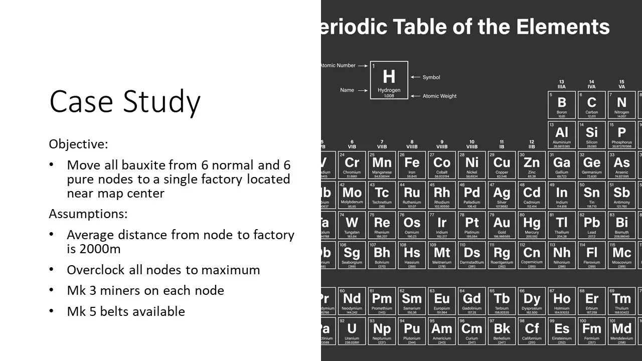
A case study is included, showing the thought process of utilizing the spreadsheet information to choose a good course of action when faced with the objective of moving all bauxite from normal and pure nodes to a factory centrally located on the map.
Introducción
This guide is about making good choices for transportation. Satisfactory is a numbers game, so I’ve crunched a lot of numbers for you to help you understand your options, how to score the costs and the benefits, and how to make a more informed choice that you can be happy with.
As with my previous guide, this is aimed at people who want to plan a little more, be frustrated a little less, and have a lot more fun. Si quieres, just to go in and try things without knowing the numbers and having a deeper understanding, please pass on by and don’t troll the rest of us with negative comments.
For everyone else who is still reading, please let me know how I can improve the guide or the companion spreadsheet. Aesthetics are not my strength, but I am very confident in the calculations.
You can find the Excel version of the spreadsheet at this enlace (Microsoft OneDrive).
I’ll put up a Google Docs version later if it doesn’t break.
Understanding the Transportation Problem
We open the map for Satisfactory and see where we’ve explored and still need to explore. But we can get an advanced look if we go to the interactive map on satisfactory-calculator.com and turn on the visibility of the various resource nodes. si lo haces, you will start to understand how resources are scattered across this massive map.
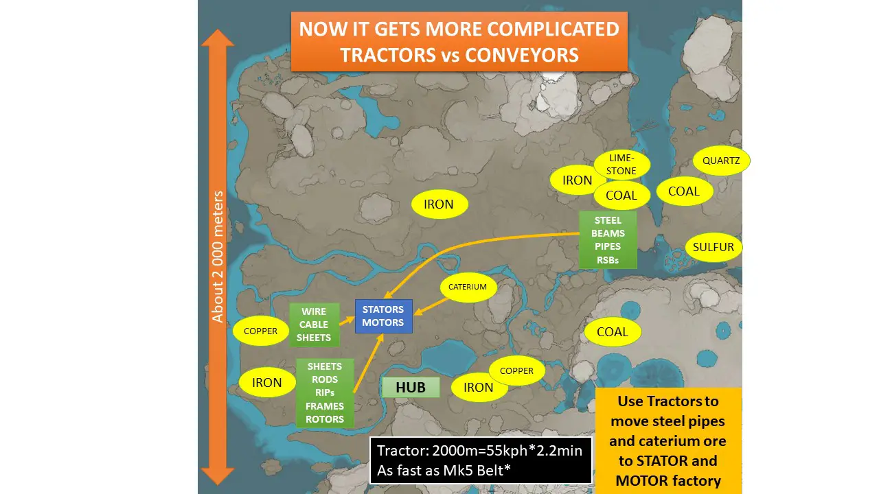
If we choose the Rocky Desert as our starting location, we might zoom in on this 2000m by 2000m area of the map and examine what pure node resources are immediately available to us. (There are many more normal and impure nodes in view, but let’s first make a point about the highest efficiency resources.)
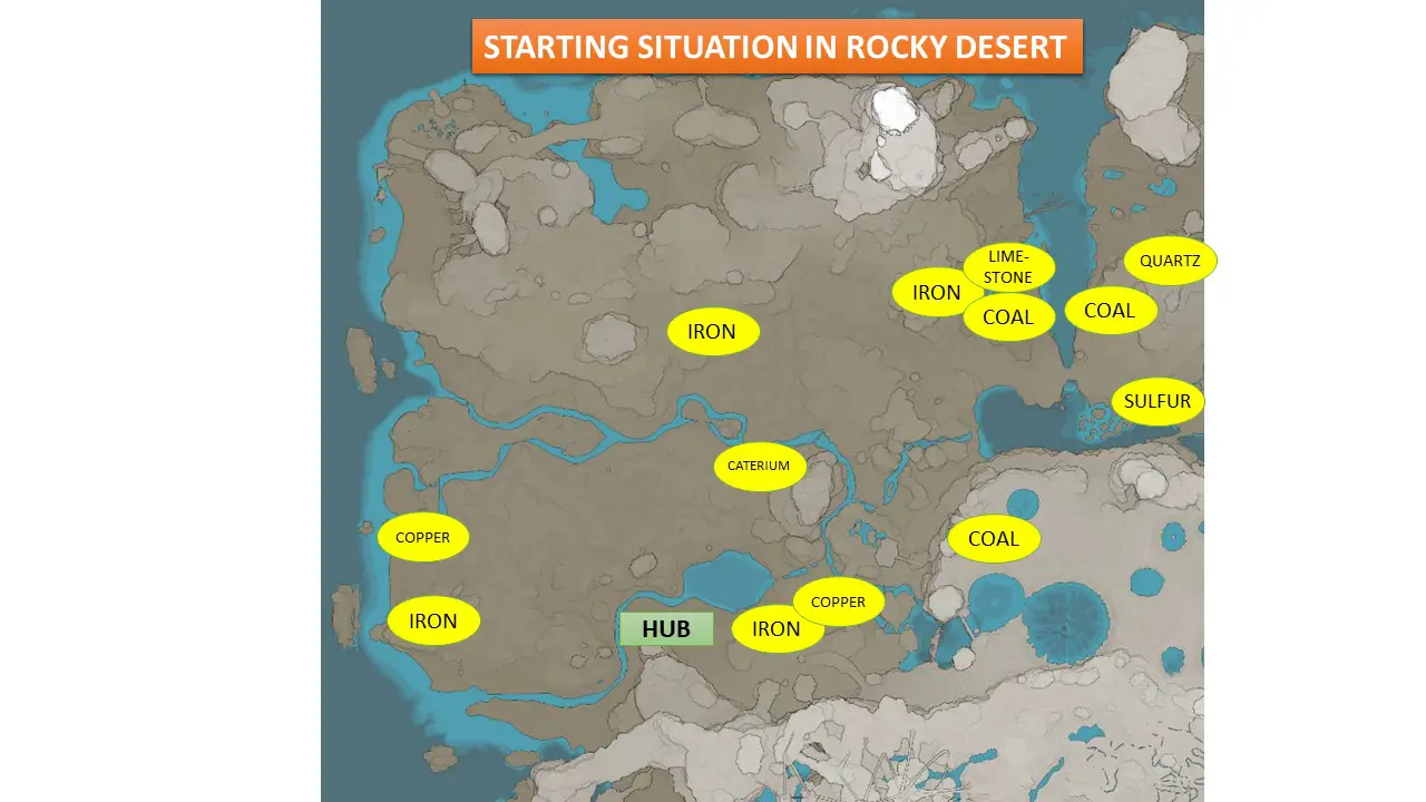
Most of what we need in early tiers is a 2500m x 1000m box rotated diagonally. What is the right way to start before fast conveyor belts and tractors? The following is how I physically distributed my first factories to be as close to the resource nodes as possible. My player character did all of the transportation by running or ziplining.
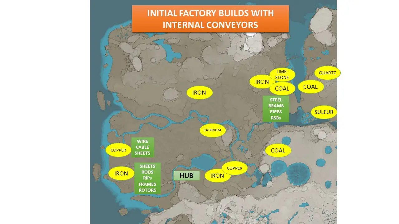
But now I needed to begin converging items from all three of these factory areas to begin making stators and motors. This presents two problems: 1) Where to put the stator-motor factory, y 2) How to move items among factories. Putting the new factory in the center would leave it 1 kilometer from the original factory areas east and west. Putting the new factory east or west, puts it 2 kilometers from the other factory.
Enter the Tractor, our first vehicle meant for automated item transportation. The Tractor can cover 2 kilometers in just 2.2 minutos, as fast as a Mk 5 belt. A lo mejor, I have Mk 3 at this time, so clearly this is a significant improvement. The upgrade path looks better as well, because Tractors can be replaced with Trucks later on, and eventually Trains.
So I used X5-Roads and the Perfect Curves tool (part of the Perfect Circle mod) to create an extensible road connecting my old factories, my HUB, and my new factories. I would later extend down to the oil patch southwest of my HUB, bringing plastic, goma, and fuel into my growing network. But all of this is a small solution to a global problem.
If we zoom out and look at the other eight 2000m by 2000m sections of the 6000m by 6000m map, now we have a wider distribution of resources, geography, and routing challenges. The idea of laying conveyor belts across kilometers of land and water is both good and bad. It’s good because conveyors do not consume power, and Mk 5 conveyors are just as fast as our Tractor at top speed. It’s bad because conveyors do not have the throughput of other options, especially when the stack size is larger than 100.
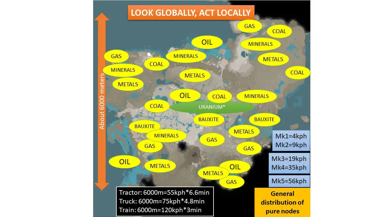
As with my previous guide, I recommend that you take as wide a view of the challenges you face from the very beginning, because you will design better solutions at the local level that fit well with world-spanning solutions that you will eventually need to create.
In these maps, I have focused on the pure nodes, because they yield the most resources for the least amount of power and building materials, which are usually scarce. When you understand your transportation options, you can make better decisions when faced with the dilemma of tapping impure nodes instead of going a little farther away to tap a normal or pure node. The next section will unlock the numbers behind your decisions.
Conveyor Belts and Vehicles, by the Numbers
En esta sección, we take the transportation numbers from the Wiki
and extend them with our own calculations.
Our first table tells us how many stacks we can move per minute given the belt tech level and stack size, and how much latency we expect for two example distances of 2000m and 6000m.
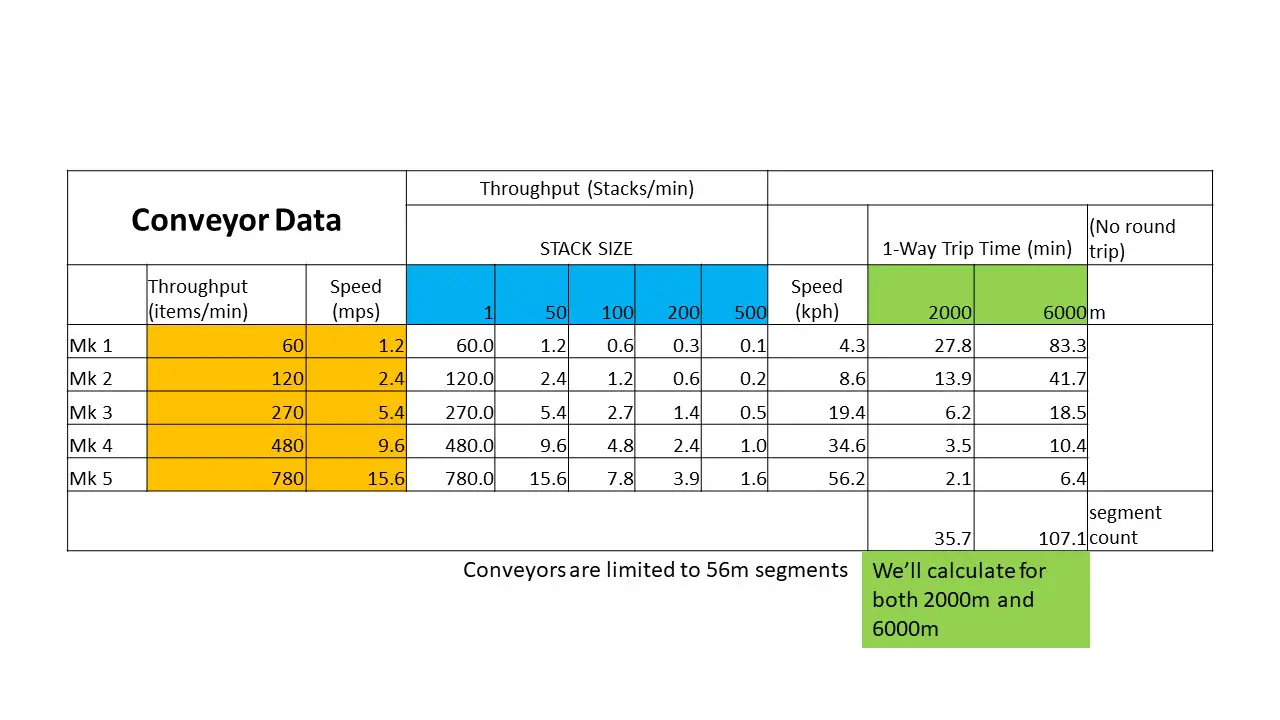
The 2000m distance comes from our starting location example, where we harvested resources from as far away as 2000m. The 6000m distance comes from a wider view of the world map, where we see the world dimensions of approximately 6000m by 6000m. Juntos, these distances are reasonable representations of regional transportation (es decir., intra-regional) and global transportation (es decir., inter-regional).
Moving to the next two tables, we calculate the benefits and cost of each vehicle type for both a 2000m one-way (4000m round trip) and 6000m one-way (12,000m round trip).

There are many variable to consider. Primero, each vehicle has a carrying capacity measured in stacks, not items. This is our first major difference with respect to conveyor belts, which move items at a fixed rate regardless of stack size.
Segundo, we make reasonable assumptions about how long a round trip will take. Every vehicle experiences a loading and unloading delay at the station, and it varies across vehicle type (drones take the longest). We can also reasonably assume that vehicles will reach their rated speed on average, because they make the round trip experiencing both uphills and downhills, always returning to the same altitude they began the route.
Tercero, we know the power requirements of the stations and the vehicles, so it is possible to compute both the fixed and the marginal energy costs of transporting items by vehicle. (Remember that conveyor belts consume zero power, so minimizing the energy cost of moving stacks is important when making a fair comparison.)
What we conclude is that any throughput number greater than 780 per minute is a benefit over using conveyor belts. We also conclude that trains are the most efficient, especially as freight wagon count increases. You may also be surprised that at 2000m, Drones are slightly more efficient than Trucks (and much more than Tractors), at a cost of moving about 30% of the Truck’s capacity.
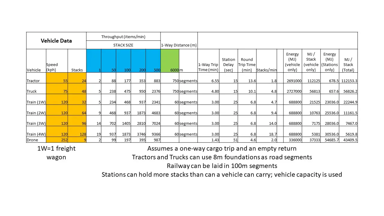
As travel distance increases, throughput drops and the energy cost per stack increases. The advantage enjoyed by trains is clear, and even the Drones increase their advantage over both Trucks and Tractors.
Our next two tables look at how long it takes to refill a vehicle station, which may constrain the actual throughput we saw in the previous two tables.
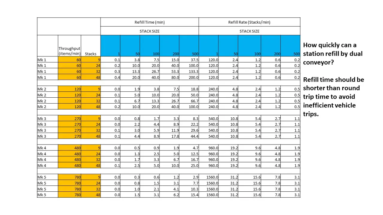
This table looks at how long it takes to refill a station *up to the capacity of the next vehicle to pick up*. (Stations generally hold more than the capacity of the vehicle, a fact that you can exploit by creating overflow (manifold) systems across multiple vehicle stations. But here we only care about filling the next vehicle, not the full station buffer.) We assume both belts are attached, for a maximum throughput (with Mk 5 cinturón) de 1560 items per minute.
On the left is the time in minutes that it takes to refill a station. A la derecha, is the refill rate in stacks per minute, not items per minute. For vehicles, stack transfer rate is all important. Por esta razón, using vehicles to transport large stack size items like wire is much more challenging, and this is why I tend to create these items within the factory they are needed, so that I can transport larger *equivalent* quantities of the input items (like ore or ingots) with my limited transportation system.
Clearly, we get the most out of our vehicle system when we can refill the stations faster than our vehicles make the round trip. For longer routes, it means we can use multiple vehicles per station. por eso, we need to know if the idle time for a vehicle at a station waiting to load is less than the round trip time, which brings us to our next table.
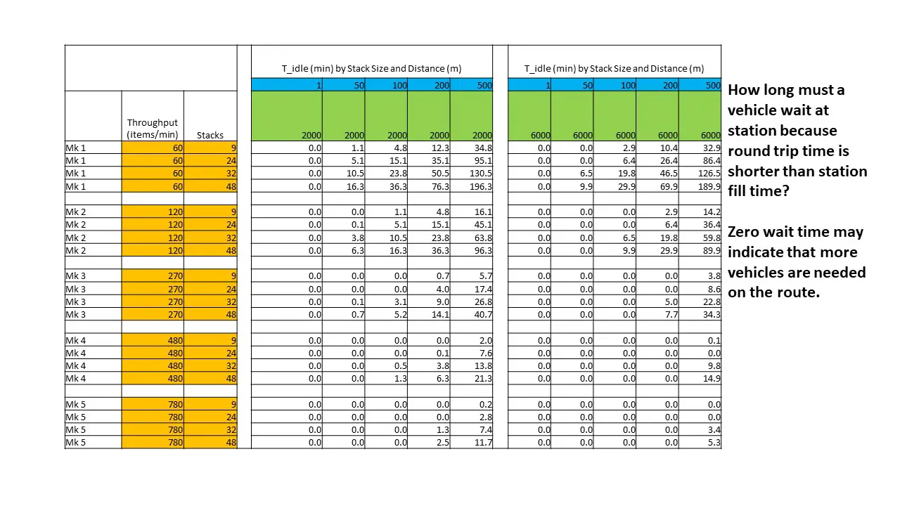
a la izquierda, calculating for a 2000m distance (4000m round trip) we see that lower-tech belts cause large wait times, especially for large stack size items (like wire). A la derecha, with a 6000m distance (12,000m round trip), these wait times are somewhat alleviated, but they are still significant for lower-tier belts.
Temprano en el juego, you will run less than full vehicles because you do not have the ability to fill the stations fast enough. As the game progresses and you tap more resource nodes with higher tier miners and use faster belts, your transportation system will begin to use up the slack and your system efficiency will increase.
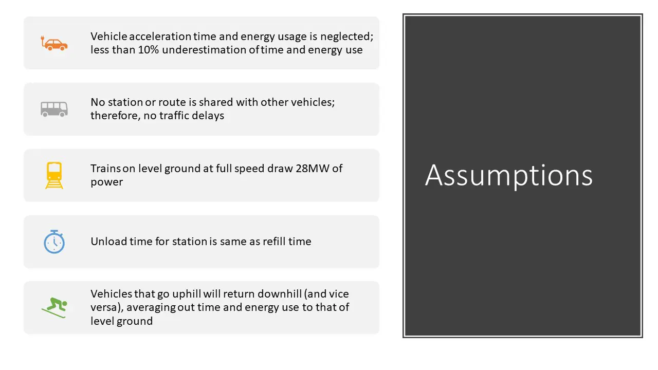
For completeness, I am disclosing the assumptions I use in my model. I think these are reasonable, but I welcome the opportunity to tweak them with your help. I have a lot of train data that I collected and analyzed and developed formulas for, but that is fodder for another guide, which I will happily contribute to if someone has already started.
Case Study: Moving Bauxite (Parte 1)
Now let’s take a real example and apply what we have learned. For this we set ourselves the task of moving all of the bauxite from normal and pure nodes to a single factory in the center of the map, where the bauxite is conveniently spread to the east and west extents of the map.
Con una excepción, all of the data in the preceding tables is used in this case study. I will call out where the exception is and point you to the spreadsheet.
Here are some additional tables either from the Wiki or built from information contained in Wiki articles, which will help us understand the challenge better and make additional calculations in the tables that follow.
One thing to remember is that Pure nodes cannot be fully exploited without a mod that gives access to faster belts. The practical effect of this is to deny access to about 1/3 of the potential output of all nodes using Mk3 miners fully overclocked.
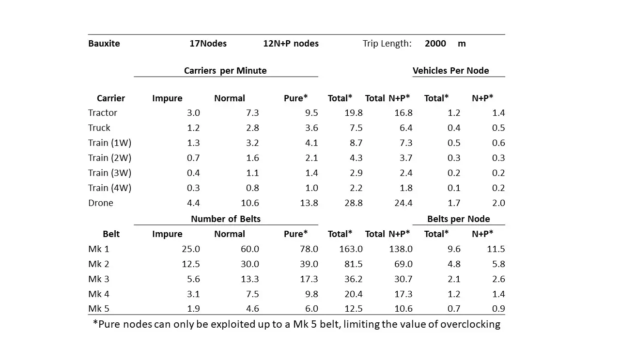
For our case study, we will use the Bauxite row in the main table.
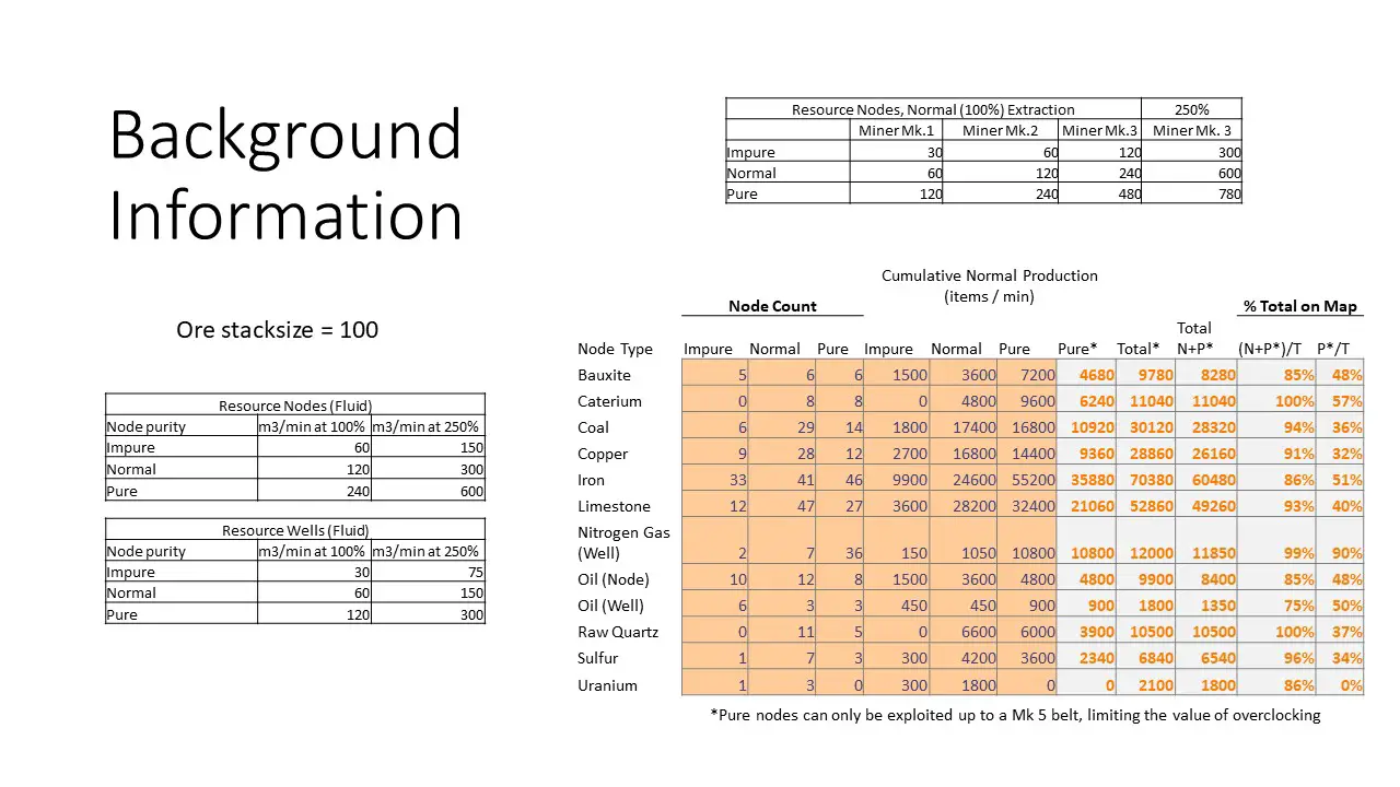
There are twelve normal and pure bauxite nodes out of a total of seventeen. In this table, we see how many vehicles (or resource «carriers») are required (como minimo) to move the total amount of bauxite from the nodes to the factory. We also compute the average number of vehicles needed per node, which is less than one for all but tractors and drones, and indicates that one carrier may be able to service multiple nodes.
We also compare these figures to the number of belts required of each tech level, so that we can make an accurate comparison of both benefits and costs. Of interest is that one Mk5 belt per node is sufficient to return all the ore to the factory.
As transportation distance increases, the number of vehicles needed increases, but the number of equivalent belts does not.
Now we start a systematic process of using the information we have calculated. This comes down to four steps.
1) Identify contraints (what we must do) and restraints (what me must not do).
2) Identify options available to us.
3) Conduct an Analysis of Alternatives to better understand the options and create evidence for decision-making.
4) Choose the Course of Action that is best for us.
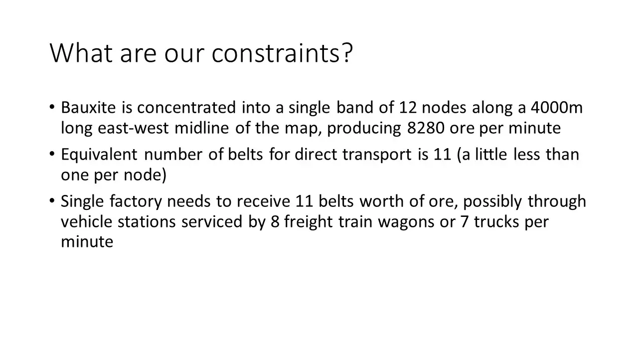
We first note where the bauxite is located on the map and in what quantities. We must adapt to where the ore is–we cannot control this fact. Además, once we decide how much ore we need, we no longer control how much quantity must be transported.
We should also be reminded that the factory will somehow need to absorb all of the ore we bring in, whether by belt or vehicle. We need to know whether we are most constrained by the number of required belts or the number of required vehicles. It is possible that the vehicles can have more throughput than we can transfer by belt, y viceversa.
There are dozens if not hundreds of possible ways of transporting items from one location to another, so we will not try to enumerate every one. We are not trying to automate the analysis process. Bastante, we are trying to train our intuition so that we don’t need to make calculations in most cases.
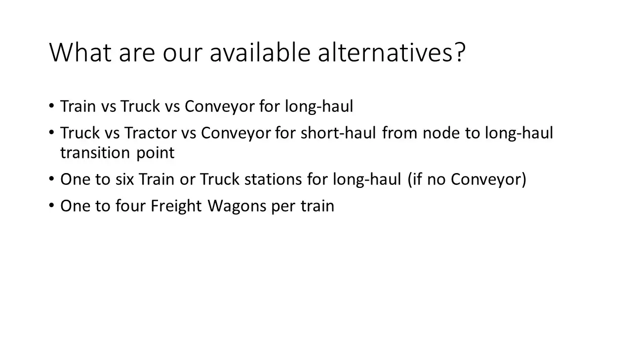
Por lo tanto, we examine the dimensions of the challenge. One way of thinking about this is to separate the long-haul from the short-haul (even if the same method is eventually used for both), how many stations we want (o necesitar) to disperse in the collection area, y (if we are running trains) how long the trains should be.
We’ll next examine the pros and cons of each dimension separately, by way of Analysis of Alternatives.
Case Study: Moving Bauxite (Parte 2)
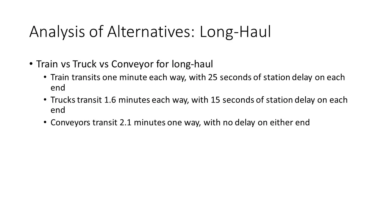
Our first Analysis of Alternatives focuses on the Long-Haul. Do we use trains, camiones, or conveyors? (Tractors are too slow and have smaller capacity compared to trucks, so we do not consider them.)
Relevant data is the round trip time and the station delay time. We see that trains are as fast as conveyors, despite traveling twice the distance. Trucks are slightly slower, but still not unreasonable. As we will see later, the main penalty to trains and trucks is the energy consumption.
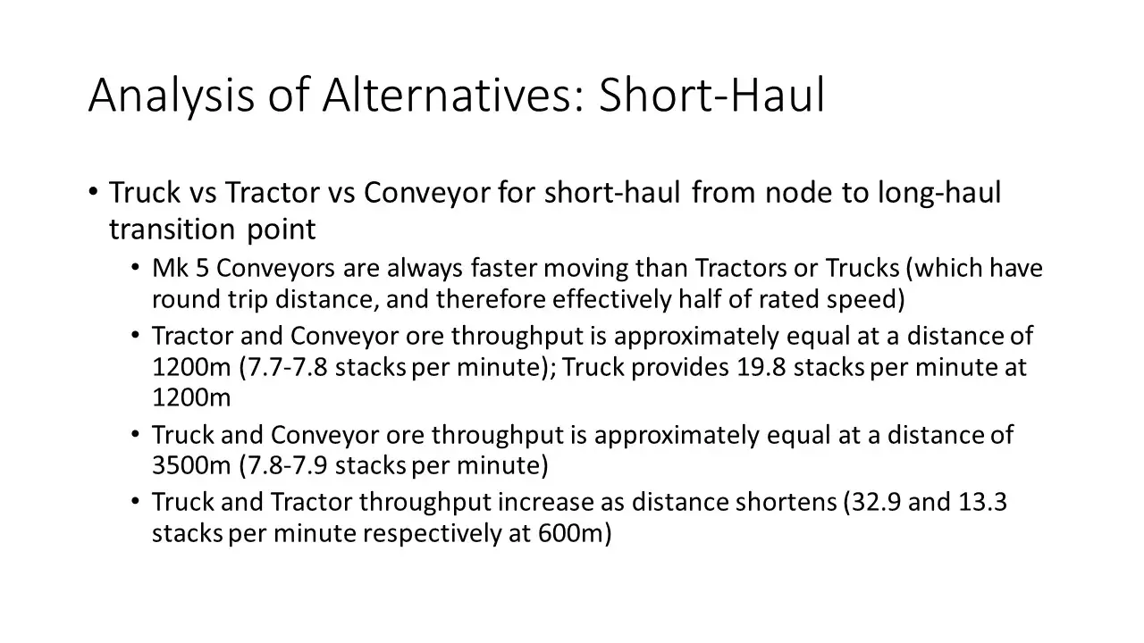
Our next analysis focuses on the Short-Haul, if we are taking a multi-modal approach (es decir., trucks deliver to trains, which deliver to the factory).
We note that Mk 5 conveyors are always faster than trucks or tractors. Because trucks and tractors make a round-trip, their average speed is half their rated speed, and this eliminates the parity between Mk 5 belts and trucks. But speed is not the primary metric. Throughput is the most important metric, and here we see that single vehicles are better than single conveyor belts.
For completeness, we show where throughput parity occurs between belts and different vehicle types. As distance increases, vehicle throughput drops, but conveyor throughput remains constant. Stack size matters greatly, with vehicles superior to belts for large stack sizes (como 500 for wire) for much longer distances.
The primary conclusion we should draw is that for short runs of 600m (we will see later where this number comes from), both trucks and tractors outperform conveyor belts at a cost of needing energy.
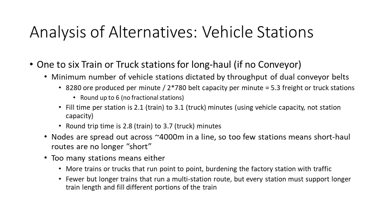
The next analysis examines the number of stations needed. There are two ways to compute this, and both ways must allow a viable solution.
Primero, we have an aggregate amount of ore to move. With only two conveyor belts for each station, whether a truck station or a freight platform, we are limited to 1560 per minute throughput at each station. De esto, we know we must have at least 6 stations or freight platforms at our factory, but we must have an equivalent (o mayor) number in the collection area as well.
Continuing with a focus on stations, we want to know how long it takes to fill the station with one vehicle’s worth of items. Trains carry 32 stacks per freight car, while trucks carry 48 stacks. Como consecuencia, the fill time is different for each type. So long as the round-trip time is greater than the fill time, our vehicles will not sit idle at the stations or run only partially full.
The second calculation determines how many and what type of vehicles are required to move the aggregate amount of ore.
If using trucks or tractors, knowing how many vehicles are required tells us how many truck stations are required. We know already that it must be at least six stations; por lo tanto, we seem to be looking at six or seven stations (unless we deliver two trucks to one of the stations) or running three tractors to each of six stations at the factory.
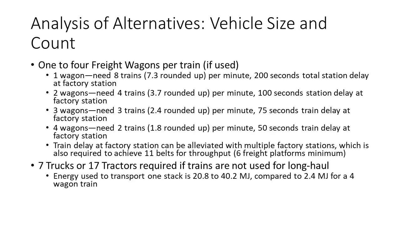
If using trains, the length of the train determines how many trains must operate. We know we need at least six freight platforms on the receiving end, and at least the same number distributed on the sending end. If we run trains with a single wagon, then we need eight trains, or about one train per 1.5 nodos. Mapping these eight trains to six stations will be somewhat challenging because of the station delay for loading/unloading as well as the limited fill/empty rate of the dual belts. We can run eight collection and receiving stations (sixteen total), one per train, but then the energy cost increases considerably.
If we move up to four-wagon trains, then we only need two trains. We have two too many freight platforms from the perspective of how fast the belts can fill and empty, but the trains need a combined total of at least eight wagons to move all of the ore because of their capacity. This is a case where the second calculation forces the solution, and why the first calculation says «al menos». (As engineers, we prefer to deal with ranges of solutions that are generally correct rather than precise point solutions that are usually wrong.)
We now have enough data to make an informed decision. Note that this process is not «push a button, look up some numbers, and get an answer» process. We are informing, not replacing, our intuition and experience. The following solution is my attempt to balance all of the factors we described above. It is not the «mejor» in any provable sense, but it is a workable solution that I can implement and manage effectively.
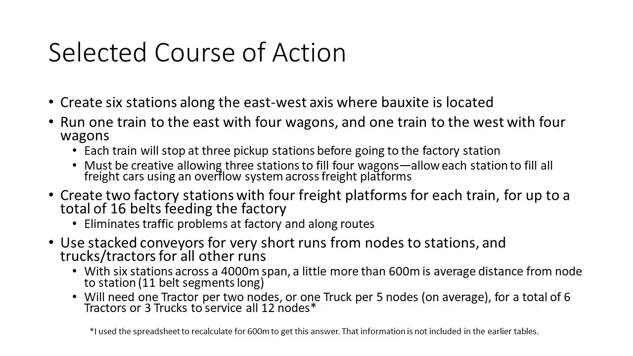
My solution is to run two trains, east and west, to collect resources from the long-haul transition points in the collection area and deliver to two independent train stations at the factory, each with four freight platforms. My spreadsheet does not explicitly compute for a multi-point route; sin embargo, this innovation will improve transit time considerably while adding only two station delays. This means the round trip time will be a little longer, but the extra freight cars will make up the throughput loss with some to spare. I rely on my solution being similar enough to what is in the spreadsheet, and this why I say the spreadsheet should inform your solution and not dictate it.
You will also note that I have a little more capacity than required (an extra belt’s worth across the stations, and an extra 0.7 freight car), which will help catch up the system when there are delays.
You also now see where the 600m distance comes from, and why I recalculated the spreadsheet for just the tractors and trucks at this distance in order to derive the needed number of each vehicle for the short-haul routes.
I have no doubt that you can come up with a better solution. The main advantage is that you now have a framework for knowing which solution is, En realidad, better for your needs and preferences.
Conclusiones
This guide is intended to help you think through your transportation challenges and bring good calculations to inform your decision-making. Al final, your needs and preferences must be compatible, so having a big-picture understanding of your options and their costs and benefits will enable you to quickly make good decisions and save time and effort in game.
My hope is that your fun playing Satisfactory will increase, and that you will achieve challenging goals with more confidence and less frustration.
If there is any way to improve this guide or the spreadsheet, please leave a comment below. This is a community guide and benefits from your constructive feedback.
Eso es todo lo que estamos compartiendo hoy para este Satisfactorio guía. Esta guía fue originalmente creada y escrita por wizard1073. En caso de que no actualicemos esta guía, puede encontrar la última actualización siguiendo este enlace.